Design and Analysis of Algorithms
II edition
Authors: Ellis Horowitz, Sartaj Sahani
Chapter -1
àWhat is an algorithm
It is defined as step by step execution of a task.
It consists of 5 steps
1.
Input: zero or more quantities are externally
supplied
2.
Output: Atleast one quantity is produced
3.
Definiteness: It is clear and unambiguous
4.
Finiteness: Algorithm may terminate after a
finite number of steps
5.
Effectiveness: Every person can easily trace the
algorithm by using pencil and paper
Algorithm syntax:
Algorithm Algorithm
name<Parameter List>
{
Body
}
Ex: Finding the maximum number in a given Array
Algorithm Max(A, n)
{
Result:=A[1];
For i:= 2 to n do
If(A[i]>result) then
Result:=A[i];
}
è
Explain in detail about Performance Analysis
(i)
Pseudocode
Conventions
Algorithm is defined
by using C language syntax
All the loops,
control statements in C language are specified to write an algorithm
Those are for loops, while,do while, if, struct, repeat
–until etc
See the syntaxes of all these in textbook
(ii)
Recursive
Algorithms
Recursion : The Function calls within itself is called
Recursion
Recursion may be two types
1.
Direct Recursion
2.
Indirect Recursion
(1)Direct Recursion:
Function calls itself is called Direct Recursion
Ex: Factorial
Algorithm fact(n)
{
If(n==0) then
Return 1;
Else return n*fact(n-1);
}
Ex: Another best Example for recursion is Towers Of Hanoi
àWhat is Time complexity
The amount of time taken to
complete an algorithm .For the finite number of iterations the amount of time
required for an algorithm is called Time complexity
In computer science, the time
complexity of an algorithm quantifies the amount of time taken by an algorithm
to run as a function of the length of the string representing the input. The
time complexity of an algorithm is commonly expressed using big O notation
àWhat is Space Complexity
Space complexity is a measure of
the amount of working storage an algorithm needs. That means how much memory,
in the worst case, is needed at any point in the algorithm.
àAnalysis of Algorithm
Algorithm can be defined in two
different ways
(1)
Priori Analysis
(2)
Posterior
Analysis
- Priori Analysis − This is a theoretical analysis of an algorithm. Efficiency of an algorithm is measured by assuming that all other factors, for example, processor speed, are constant and have no effect on the implementation.
- Posterior Analysis − This is an empirical analysis of an algorithm. The selected algorithm is implemented using programming language. This is then executed on target computer machine. In this analysis, actual statistics like running time and space required, are collected.
àAsymptotic Notations
O-notation:
To denote asymptotic upper bound, we use O-notation. For a given function g(n), we denote by O(g(n)) (pronounced “big-oh of g of n”) the set of functions:
O(g(n))= { f(n) : there exist positive constants c and n0 such that
To denote asymptotic upper bound, we use O-notation. For a given function g(n), we denote by O(g(n)) (pronounced “big-oh of g of n”) the set of functions:
O(g(n))= { f(n) : there exist positive constants c and n0 such that
Ω-notation:
To denote asymptotic lower bound, we use Ω-notation. For a given function g(n), we denote by Ω(g(n)) (pronounced “big-omega of g of n”) the set of functions:
Ω(g(n))= { f(n) : there exist positive constants c and n0 such that
To denote asymptotic lower bound, we use Ω-notation. For a given function g(n), we denote by Ω(g(n)) (pronounced “big-omega of g of n”) the set of functions:
Ω(g(n))= { f(n) : there exist positive constants c and n0 such that
Θ-notation:
To denote asymptotic tight bound, we use Θ-notation. For a given function g(n), we denote by Θ(g(n)) (pronounced “big-theta of g of n”) the set of functions:
Θ(g(n))= { f(n) : there exist positive constants c1,c2 and n0 such that 0≤c1∗g(n)≤f(n)≤c2∗g(n) for all n>n0}
To denote asymptotic tight bound, we use Θ-notation. For a given function g(n), we denote by Θ(g(n)) (pronounced “big-theta of g of n”) the set of functions:
Θ(g(n))= { f(n) : there exist positive constants c1,c2 and n0 such that 0≤c1∗g(n)≤f(n)≤c2∗g(n) for all n>n0}
Chapter -3 Divide and conquer
Many algorithms are recursive in nature to solve a given problem recursively dealing with sub-problems.
In divide and conquer approach, a problem is divided into smaller problems, then the smaller problems are solved independently, and finally the solutions of smaller problems are combined into a solution for the large problem.
Generally, divide-and-conquer algorithms have three parts −
- Divide the problem into a number of sub-problems that are smaller instances of the same problem.
- Conquer the sub-problems by solving them recursively. If they are small enough, solve the sub-problems as base cases.
- Combine the solutions to the sub-problems into the solution for the original problem.
Application of Divide and Conquer Approach
Following are some problems, which are solved using divide and conquer approach.- Finding the maximum and minimum of a sequence of numbers
- Strassen’s matrix multiplication
- Merge sort
- Binary search
Binary Search
Algorithm Bsearch(a, n,x)
{
low:=1;
high:=n;
mid=low+high/2;
if low ≤ high then
mid = (low + high) / 2
if x = S[mid] then
return mid
elsif x < s[mid] then
high=mid-1;
else
low=mid+1;
else
return x
In case of Binary search, the number of element comparisions for successful
search is the total number of comparisions for n elements summing and divided by n .
we will get the maximum of 4 comparisions and the minimum of 1 comparision
Average number of comparisions for the binary search is 3.21 approximately
Example and The time complexity of Binary search is seen in notebook
For successful search
. . Best O(1)
. Average O(log n)
. Worst O(log n)
For unsuccessful Search
Best, Average, worst is O(logn)
Quick Sort
Quicksort is a divide and conquer algorithm. Quicksort first divides a large array into two smaller sub-arrays: the low elements and the high elements. Quicksort can then recursively sort the sub-arrays.
The steps are:
- Pick an element, called a pivot, from the array.
- Partitioning: reorder the array so that all elements with values less than the pivot come before the pivot, while all elements with values greater than the pivot come after it (equal values can go either way). After this partitioning, the pivot is in its final position. This is called the partition operation.
- Recursively apply the above steps to the sub-array of elements with smaller values and separately to the sub-array of elements with greater values
1. low --> Starting index, high --> Ending index */
2. Algorithm quickSort(arr[], low, high)
3. {
4. if (low < high)
5. {
6. /* pi is partitioning index, arr[p] is now
7. at right place */
8. pi = partition(arr, low, high);
9.
10. quickSort(arr, low, pi - 1); // Before pi
11. quickSort(arr, pi + 1, high); // After pi
12. }
13. }
Worst-case:
O(N2)
This happens when the pivot is the smallest (or the largest)
element.
Then one of the partitions is empty, and we repeat
recursively the procedure for N-1 elements.
Best-case
O(NlogN)
The best case is when the pivot is the median of the array,
and then the left and the right part will have same size.
There are logN partitions, and to obtain each partitions we
do N comparisons
(and not more than N/2 swaps). Hence the complexity is
O(NlogN)
Average-caseO(NlogN)
Advantages - :One of the fastest algorithms on
average.
 Time complexities of quick sort can be seen in notebook
Merge sort:
Merge sort is based on the divide-and-conquer paradigm. Its worst-case running time
has a lower order of growth than insertion sort. Since we are dealing with subproblems, we state each subproblem as sorting
a subarray A[p .. r]. Initially, p = 1 and
r = n, but these values change as we recurse through subproblems.
To sort A[p .. r]:
1. Divide Step
If a given array A has zero or one element, simply return; it
is already sorted. Otherwise, split A[p .. r] into two subarrays
A[p .. q] and A[q + 1 .. r],
each containing about half of the elements of A[p .. r]. That is,
q is the halfway point of A[p .. r].
2. Conquer Step
Conquer by recursively sorting the two subarrays A[p ..
q] and A[q + 1 .. r].
3. Combine Step
Combine the elements back in A[p .. r] by merging the two sorted subarrays
A[p .. q] and A[q + 1 .. r]
into a sorted sequence. To accomplish this step, we will
define a procedure MERGE (A, p, q, r).
Note that the recursion bottoms out when the subarray has just
one element, so that it is
trivially sorted.
Analyzing Merge Sort
For simplicity, assume that n is a power of 2 so that each divide step yields two subproblems, both of size exactly
n/2.
The base case occurs when n = 1.
When n ≥ 2, time for merge sort steps:
-
Divide: Just compute q as the average of p and r, which takes constant time i.e. Θ(1).
-
Conquer: Recursively solve 2 subproblems, each of size n/2, which is 2T(n/2).
-
Combine: MERGE on an n-element subarray takes Θ(n) time.
Merging
What remains is the MERGE procedure. The following is the
input and output of the MERGE procedure.
INPUT: Array A and indices
p, q, r such that p ≤ q ≤ r and subarray
A[p .. q]
is sorted and subarray A[q + 1 .. r] is sorted. By restrictions on
p, q, r,
neither subarray is empty.
OUTPUT: The two subarrays are merged into a single sorted subarray in
A[p ..
r].
We implement it so that it takes Θ(n) time, where
n = r − p + 1, which is the
number of elements being merged.
Merging two sorted subarrays Algorithm
Algorithm
Merge(low,mid,high)
{
h:=low,i:=low;j:=mid+1;
while(h<=mid)
and (j<=high)) do
{
if((a[h]<=a[j]) then
{
b[i]:=a[h];
h:=h+1;
}
else
{
b[i]:=a[j];
j=j+1;
}
i=i+1;
}
if((h>mid)
then
for
k:=j to high do
{
b[i]:=a[k];
i:=i+1;
}
else
for
k:=h to mid do
{
b[i]:=a[k];i:=i+1;
}
for
k:=low to high do
a[k]:=b[k];
}
Merge sort Algorithm
Algorithm
mergesort(low,high)
{
If(low<high)then
{
Mid=(low+high)/2;
mergesort(low,mid)
mergesort(low+1,high)
}
}Chapter-4 :Greeedy method
In divide and conquer, the problems which are large we can divide the problems into subproblems.When the array size is large, we can divide those problems into subproblems .recursively apply the divide and conquer method to each set and finally merge the problems
But in some cases, we cannot divide the problems into subproblems
Ex:Knapsack
These type of problems depend on the optimality (i.e either minimum or maximim)
Feasiblity:
the set of all possible solution taken under a given problem criteria is called feasiblity
Ex:= let z=3x+4y
if 0<x<1 , -1<y<1
therefore x=(0,1)
y=(-1,0,1)
Substitute x and y values in above equation
the possibilities are{ (0,-1)(0,0)(0,1)(1,-1)(1,0)(1,1)}
All these possibilities come under feasibility
Optimality
The possible solution taken from given sets is called optimality
i.e either minimum or maximum based on the given problem
(1,1) gives the optimal solution for the above problem
Knapsack problem
In this context, the items should be selected in such a way that the thief will carry those items for which he will gain maximum profit. Hence, the objective of the thief is to maximize the profit.
In this case, items can be broken into smaller pieces, hence the thief can select fractions of items.
According to the problem statement,
- There are n items in the store
- Weight of ith item
wi>0
- and
- Capacity of the Knapsack is W
The ith item contributes the weight
to the total weight in the knapsack and profit
Hence, the objective of this algorithm is to
kanpsack Problem see in notes
-->Minimum cost spanning trees
What is a Spanning Tree?
Given an undirected and connected graph G=(V,E)
, a spanning tree of the graph G is a tree that spans G (that is, it includes every vertex of G) and is a subgraph of G (every edge in the tree belongs to G
What is a Minimum Spanning Tree?
The cost of the spanning tree is the sum of the weights of all the edges in the tree. There can be many spanning trees. Minimum spanning tree is the spanning tree where the cost is minimum among all the spanning trees. There also can be many minimum spanning trees.
Prim’s Algorithm
Prim’s Algorithm also use Greedy approach to find the minimum spanning tree. In Prim’s Algorithm we grow the spanning tree from a starting position. Unlike an edge in Kruskal's, we add vertex to the growing spanning tree in Prim's.Algorithm Steps:
- Maintain two disjoint sets of vertices. One containing vertices that are in the growing spanning tree and other that are not in the growing spanning tree.
- Select the cheapest vertex that is connected to the growing spanning tree and is not in the growing spanning tree and add it into the growing spanning tree. This can be done using Priority Queues. Insert the vertices, that are connected to growing spanning tree, into the Priority Queue.
- Check for cycles. To do that, mark the nodes which have been already selected and insert only those nodes in the Priority Queue that are not marked.
Kruskal’s Algorithm
Kruskal’s Algorithm builds the spanning tree by adding edges one by one into a growing spanning tree. Kruskal's algorithm follows greedy approach as in each iteration it finds an edge which has least weight and add it to the growing spanning tree.Algorithm Steps:
- Sort the graph edges with respect to their weights.
- Start adding edges to the MST from the edge with the smallest weight until the edge of the largest weight.
- Only add edges which doesn't form a cycle , edges which connect only disconnected components.
Now pick all edges one by one from sorted list of edges
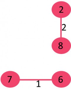
1. Pick edge 7-6: No cycle is formed, include it.

2. Pick edge 8-2: No cycle is formed, include it.
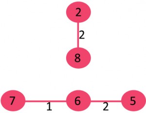
3. Pick edge 6-5: No cycle is formed, include it.
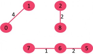
4. Pick edge 0-1: No cycle is formed, include it.
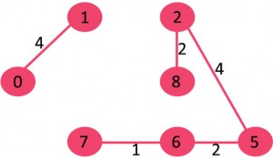
5. Pick edge 2-5: No cycle is formed, include it.
6. Pick edge 8-6: Since including this edge results in cycle, discard it.
7. Pick edge 2-3: No cycle is formed, include it.
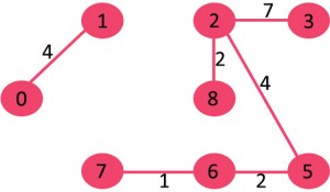
8. Pick edge 7-8: Since including this edge results in cycle, discard it.
9. Pick edge 0-7: No cycle is formed, include it.
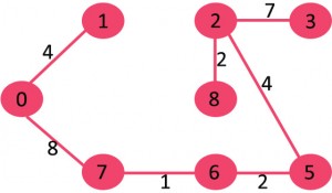
10. Pick edge 1-2: Since including this edge results in cycle, discard it.
11. Pick edge 3-4: No cycle is formed, include it.
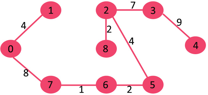
Since the number of edges included equals (V – 1), the algorithm stops here.
1. Pick edge 7-6: No cycle is formed, include it.
2. Pick edge 8-2: No cycle is formed, include it.

3. Pick edge 6-5: No cycle is formed, include it.

4. Pick edge 0-1: No cycle is formed, include it.

5. Pick edge 2-5: No cycle is formed, include it.

6. Pick edge 8-6: Since including this edge results in cycle, discard it.
7. Pick edge 2-3: No cycle is formed, include it.

8. Pick edge 7-8: Since including this edge results in cycle, discard it.
9. Pick edge 0-7: No cycle is formed, include it.

10. Pick edge 1-2: Since including this edge results in cycle, discard it.
11. Pick edge 3-4: No cycle is formed, include it.

Since the number of edges included equals (V – 1), the algorithm stops here.
chapter-5 Dynamic programming
Dynamic Programming
Dynamic Programming is mainly an optimization over plain recursion. Wherever we see a recursive solution that has repeated calls for same inputs, we can optimize it using Dynamic Programming. The idea is to simply store the results of subproblems, so that we do not have to re-comupute them when needed later. This simple optimization reduces time complexities from exponential to polynomial. For example, if we write simple recursive solution for Fibonacci Numbers, we get exponential time complexity and if we optimize it by storing solutions of subproblems, time complexity reduces to linear.
Optimal binary search trees
Given a sorted array keys[0.. n-1] of search keys and an array freq[0.. n-1] of frequency counts, where freq[i] is the number of searches to keys[i]. Construct a binary search tree of all keys such that the total cost of all the searches is as small as possible.
Let us first define the cost of a BST. The cost of a BST node is level of that node multiplied by its frequency. Level of root is 1.
Example 1
Input:  keys[] = {10, 12}, freq[] = {34, 50}
There can be following two possible BSTs
        10                       12
          \                     /
           12                 10
          I                     II
Frequency of searches of 10 and 12 are 34 and 50 respectively.
The cost of tree I is 34*1 + 50*2 = 134
The cost of tree II is 50*1 + 34*2 = 118

Example 2
Input:  keys[] = {10, 12, 20}, freq[] = {34, 8, 50}
There can be following possible BSTs
    10                12                 20         10              20
      \             /    \              /             \            /
      12          10     20           12               20         10
        \                            /                 /           \
         20                        10                12             12
     I               II             III             IV             V
Among all possible BSTs, cost of the fifth BST is minimum.
Cost of the fifth BST is 1*50 + 2*34 + 3*8 = 142
Optimal Substructure:
The optimal cost for freq[i..j] can be recursively calculated using following formula.

The optimal cost for freq[i..j] can be recursively calculated using following formula.
We need to calculate optCost(0, n-1) to find the result.
The idea of above formula is simple, we one by one try all nodes as root (r varies from i to j in second term). When we make rth node as root, we recursively calculate optimal cost from i to r-1 and r+1 to j.
We add sum of frequencies from i to j (see first term in the above formula), this is added because every search will go through root and one comparison will be done for every search
FLOWSHOP SCHEDULING
- Flow shop scheduling problems are a class of scheduling problems with a workshop or group shop.
- If there is more than one machine and there are multiple jobs, then each job must be processed by corresponding machine or processor.
- That means with operation of each job must be processed on.
- Flow shop scheduling is a special case of job scheduling where there is strict order of all operations to be performed on all jobs.
- Solution methods of Flow shop scheduling are Branch and Bound, Dynamic programming, Heuristic algorithm and Meta-heuristics.
Example:
Schedule two jobs on 4 machine using flow shop scheduling technique. The time required by each operation of these jobs is given by following matrix.
The sequencing problem can be stated as determining a sequence S such that one or several sequencing objectives are optimized.
- (Average)Flow time,
- Makespan,Cmax
- (Average) Tardiness,
Traversal Techniques
Tree Traversals (Inorder, Preorder and Postorder)
Unlike linear data structures (Array, Linked List, Queues, Stacks, etc) which have only one logical way to traverse them, trees can be traversed in different ways. Following are the generally used ways for traversing trees.

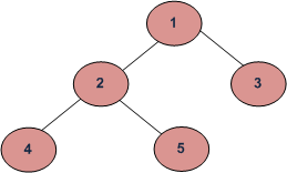
Example Tree
Depth First Traversals:
(a) Inorder (Left, Root, Right) : 4 2 5 1 3
(b) Preorder (Root, Left, Right) : 1 2 4 5 3
(c) Postorder (Left, Right, Root) : 4 5 2 3 1
(a) Inorder (Left, Root, Right) : 4 2 5 1 3
(b) Preorder (Root, Left, Right) : 1 2 4 5 3
(c) Postorder (Left, Right, Root) : 4 5 2 3 1
Breadth First or Level Order Traversal : 1 2 3 4 5
Inorder Traversal (Practice):
Algorithm Inorder(tree)
   1. Traverse the left subtree, i.e., call Inorder(left-subtree)
   2. Visit the root.
   3. Traverse the right subtree, i.e., call Inorder(right-subtree)
Uses of Inorder
In case of binary search trees (BST), Inorder traversal gives nodes in non-decreasing order. To get nodes of BST in non-increasing order, a variation of Inorder traversal where Inorder traversal s reversed can be used.
Example: Inorder traversal for the above-given figure is 4 2 5 1 3.
In case of binary search trees (BST), Inorder traversal gives nodes in non-decreasing order. To get nodes of BST in non-increasing order, a variation of Inorder traversal where Inorder traversal s reversed can be used.
Example: Inorder traversal for the above-given figure is 4 2 5 1 3.
Preorder Traversal :
Algorithm Preorder(tree)
   1. Visit the root.
   2. Traverse the left subtree, i.e., call Preorder(left-subtree)
   3. Traverse the right subtree, i.e., call Preorder(right-subtree)
Uses of Preorder
Preorder traversal is used to create a copy of the tree. Preorder traversal is also used to get prefix expression on of an expression tree.
Example: Preorder traversal for the above given figure is 1 2 4 5 3.
Preorder traversal is used to create a copy of the tree. Preorder traversal is also used to get prefix expression on of an expression tree.
Example: Preorder traversal for the above given figure is 1 2 4 5 3.
Postorder Traversal
Algorithm postorder(tree)
1. Traverse the left subtree i.e call postOrder(left-subtree)
2. Traverse the right subtree i.e call postOrder(right-subtree)
3. visit the root


No comments:
Post a Comment